3 Results
3.1 Simulations
The constant treatment effect approach outperformed other approaches in the base case scenario (N = 4,250; OR = 0.8; AUC= 0.75; no absolute treatment harm) with a true constant treatment effect (median RMSE: constant treatment effect 0.009; linear interaction 0.014; RCS-3 0.018). The linear interaction model was optimal under true linear deviations (median RMSE: constant treatment effect 0.027; linear interaction 0.015; RCS-3 0.018; Figure \(\ref{fig:rmsebase}\) panels A-C) and even in the presence of true quadratic deviations (median RMSE: constant treatment effect 0.057; linear interaction 0.020; RCS-3 0.021; Figure \(\ref{fig:rmsebase}\) panels A-C) from a constant relative treatment effect. With non-monotonic deviations, RCS-3 slightly outperformed the linear interaction model (Median RMSE: linear interaction 0.019; RCS-3 0.018; Figure \(\ref{fig:rmsebase}\) panel D). With strong treatment-related harms the results were very similar in most scenarios (Figure \(\ref{fig:rmsebase}\) panels A-C). Under non-monotonic deviations the optimal performance of RCS-3 was more pronounced (Median RMSE: linear interaction 0.024; RCS-3 0.019; Figure \(\ref{fig:rmsebase}\) panel D). A stronger average treatment effect (OR=0.5) led to larger absolute benefit predictions and consequently to larger RMSE for all approaches, but the relative differences between different approaches were similar to the base case scenario (Supplement, Figure S10).
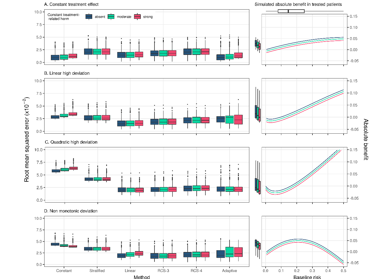
Figure 3.1: RMSE of the considered methods across 500 replications calculated from a simulated super-population of size 500,000. The scenario with true constant relative treatment effect (panel A) had a true prediction AUC of 0.75 and sample size of 4250. The RMSE is also presented for strong linear (panel B), strong quadratic (panel C), and non-monotonic (panel D) from constant relative treatment effects. Panels on the right side present the true relations between baseline risk (x-axis) and absolute treatment benefit (y-axis). The 2.5, 25, 50, 75, and 97.5 percentiles of the risk distribution are expressed by the boxplot on the top. The 2.5, 25, 50, 75, and 97.5 percentiles of the true benefit distributions are expressed by the boxplots on the side of the right-handside panel.
The adaptive approach had limited loss of performance in terms of the median RMSE to the best-performing method in each scenario. However, compared to the best-performing approach, its RMSE was more variable in scenarios with linear and non-monotonic deviations, especially when also including moderate or strong treatment-related harms. On closer inspection, we found that this behavior was caused by selecting the constant treatment effect model in a substantial proportion of the replications (Supplement, Figure S3).
Increasing the sample size to 17,000 favored RCS-3 the most. The difference in performance with the linear interaction approach was more limited in settings with a constant treatment effect (Median RMSE: linear interaction 0.007; RCS-3 0.009) and with a true linear interaction (Median RMSE: linear interaction 0.008; RCS-3 0.009). and more emphasized in settings with strong quadratic deviations (Median RMSE: linear interaction 0.013; RCS-3 0.011) and non-monotonic deviations (Median RMSE: linear interaction 0.014; RCS-3 0.010). Due to the large sample size, the RMSE of the adaptive approach was even more similar to the best-performing method, and the constant relative treatment effect model was less often wrongly selected (Supplement, Figure S4).
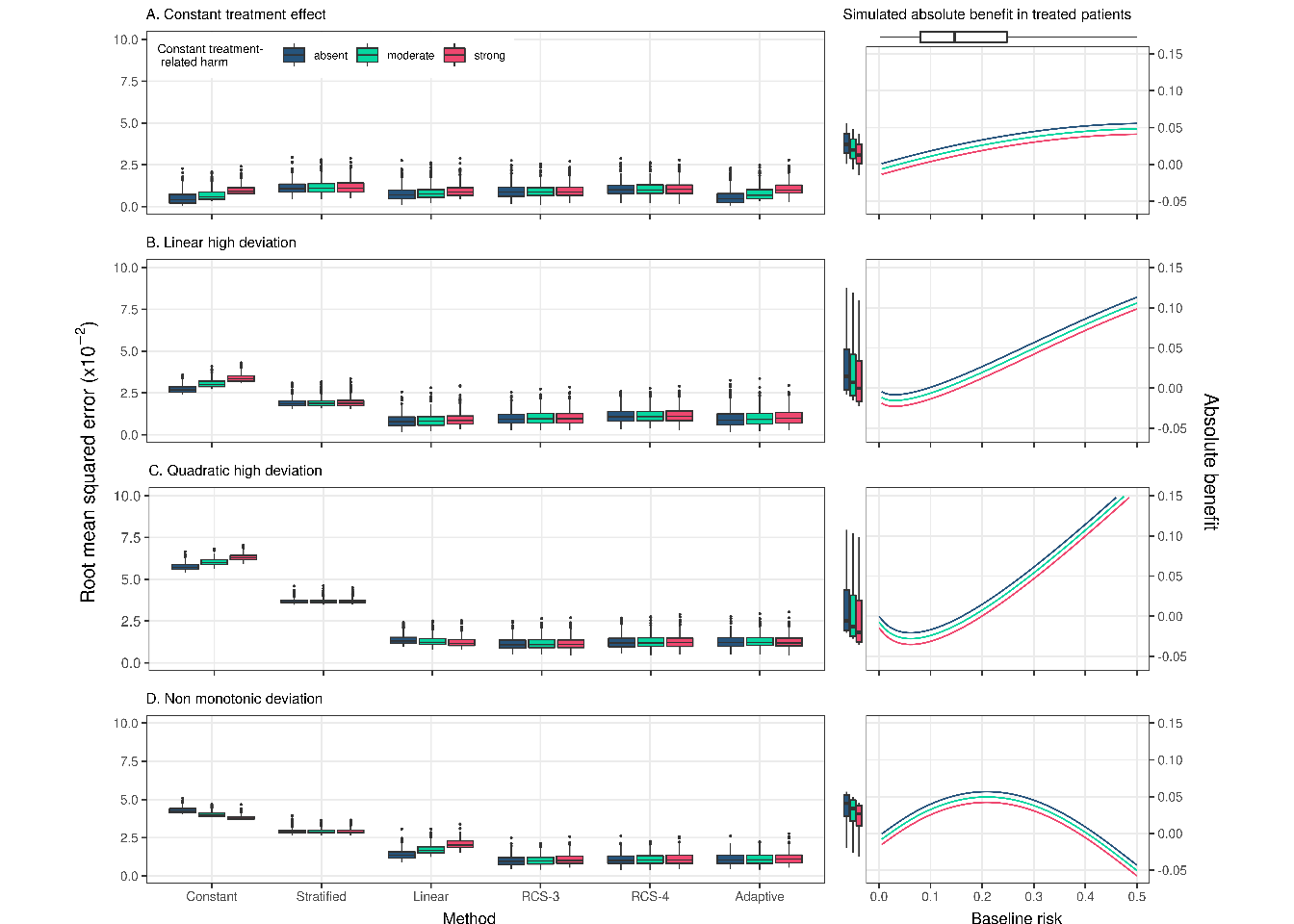
Figure 3.2: RMSE of the considered methods across 500 replications calculated in simulated samples of size 17,000 rather than 4,250 in Figure \(\ref{fig:rmsebase}\). RMSE was calculated on a super-population of size 500,000
Similarly, when we increased the AUC of the true prediction model to 0.85 (OR = 0.8 and N = 4,250), RCS-3 had the lowest RMSE in the case of strong quadratic or non-monotonic deviations and very comparable performance to the – optimal – linear interaction model in the case of strong linear deviations (median RMSE of 0.016 for RCS-3 compared to 0.014 for the linear interaction model). Similar to the base case scenario the adaptive approach wrongly selected the constant treatment effect model (23% and 25% of the replications in the strong linear and non-monotonic deviation scenarios without treatment-related harms, respectively), leading to increased variability of the RMSE (Supplement, Figure S5).
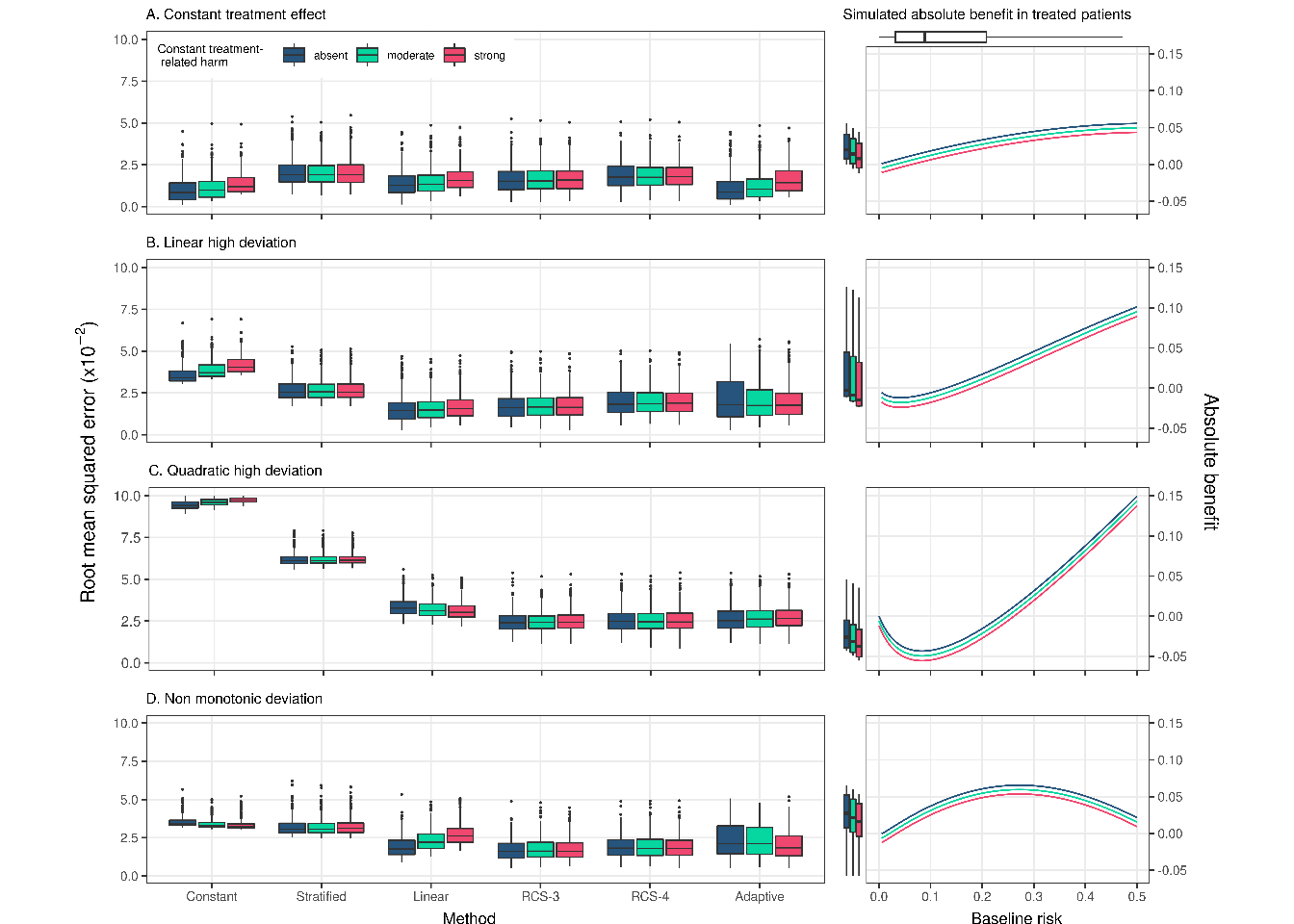
Figure 3.3: RMSE of the considered methods across 500 replications calculated in simulated samples 4,250. True prediction AUC of 0.85. RMSE was calculated on a super-population of size 500,000
With a true constant relative treatment effect, discrimination for benefit was only slightly lower for the linear interaction model, but substantially lower for the non-linear RCS approaches (Figure \(\ref{fig:discrimination}\); panel A). With strong linear or quadratic deviations from a constant relative treatment effect, all methods discriminated quite similarly (Figure \(\ref{fig:discrimination}\); panels B-C). With non-monotonic deviations, the constant effect model had much lower discriminative ability compared to all other methods (median AUC of 0.500 for the constant effects model, 0.528 for the linear interaction model and 0.530 Figure \(\ref{fig:discrimination}\); panel D). The adaptive approach was unstable in terms of discrimination for benefit, especially with treatment-related harms. With increasing number of RCS knots, we observed decreasing median values and increasing variability of the c-for-benefit in all scenarios. When we increased the sample size to 17,000 we observed similar trends, however the performance of all methods was more stable (Supplement, Figure S6). Finally, when we increased the true prediction AUC to 0.85 the adaptive approach was, again, more conservative, especially with non-monotonic deviations and null or moderate treatment-related harms (Supplement, Figure S5).
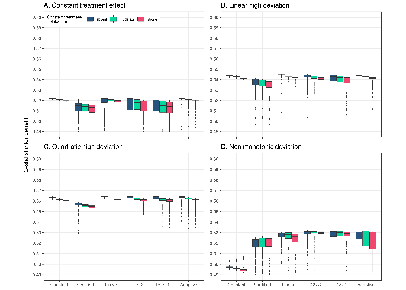
Figure 3.4: Discrimination for benefit of the considered methods across 500 replications calculated in a simulated samples of size 4,250. True prediction AUC of 0.75.
In terms of calibration for benefit, the constant effects model outperformed all other models in the scenario with true constant treatment effects, but was miscalibrated for all deviation scenarios (Figure \(\ref{fig:calibration}\)). The linear interaction model showed best or close to best calibration across all scenarios and was only outperformed by RCS-3 in the case of non-monotonic deviations and treatment-related harms (Figure \(\ref{fig:calibration}\); panel D). The adaptive approach was worse calibrated under strong linear and non-monotonic deviations compared to the linear interaction model and RCS-3. When we increased the sample size to 17,000 (Supplement, Figure S6) or the true prediction AUC to 0.85 (Supplement, Figure S7), RCS-3 was somewhat better calibrated than the linear interaction model with strong quadratic deviations.
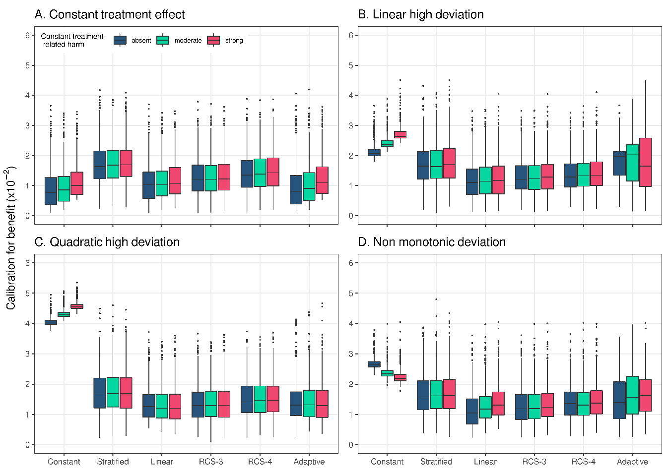
Figure 3.5: Calibration for benefit of the considered methods across 500 replications calculated in a simulated sample of size 500,000. True prediction AUC of 0.75 and sample size of 4,250.
The results from all individual scenarios can be explored online at https://arekkas.shinyapps.io/simulation_viewer/. Additionally, all the code for the simulations can be found at https://github.com/rekkasa/arekkas_HteSimulation_XXXX_2021
3.2 Empirical illustration
We used the derived prognostic index to fit a constant treatment effect, a linear interaction and an RCS-3 model individualizing absolute benefit predictions. Following our simulation results, RCS-4 and RCS-5 models were excluded. Finally, an adaptive approach with the 3 candidate models was applied.
All considered methods provided similar fits, predicting increasing benefits for patients with higher baseline risk predictions, and followed the evolution of the stratified estimates closely (Figure \(\ref{fig:gusto}\)). The constant treatment effect model had somewhat lower AIC compared to the linear interaction model (AIC: 9,336 versus 9,342), equal cross-validated discrimination (c-for-benefit: 0.525), and slightly better cross-validated calibration (ICI-for benefit: 0.010 versus 0.012). In conclusion, although the sample size (30,510 patients; 2,128 events) allowed for flexible modeling approaches, a simpler constant treatment effect model is adequate for predicting absolute 30-day mortality benefits of treatment with tPA in patients with acute MI.
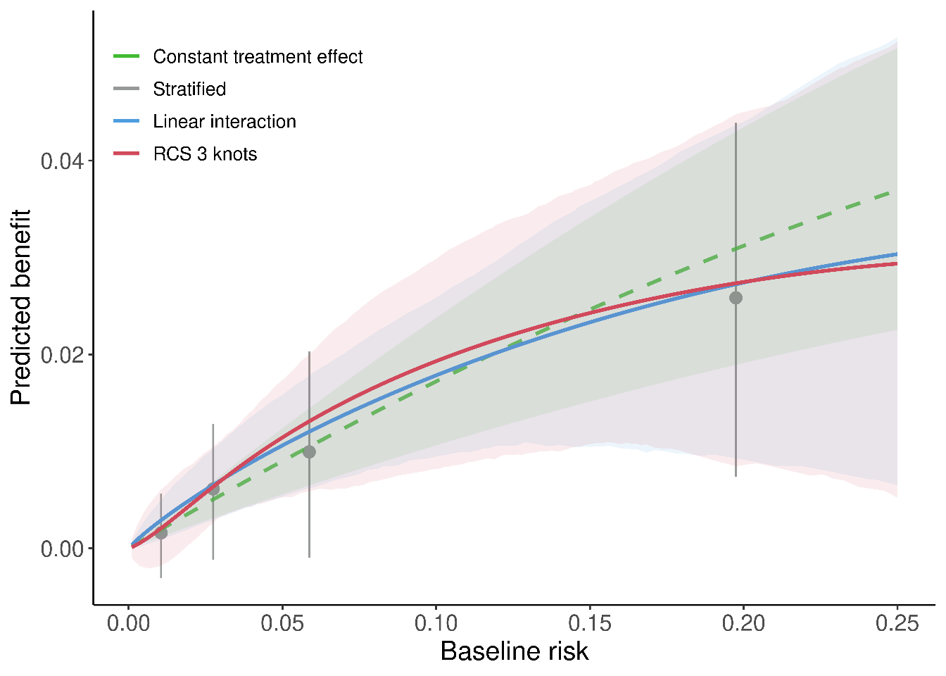
Figure 3.6: Individualized absolute benefit predictions based on baseline risk when using a constant treatment effect approach, a linear interaction approach and RCS smoothing using 3 knots. Risk stratified estimates of absolute benefit are presented within quartiles of baseline risk as reference.